Quick start

Start nnitp by entering this command:

nnitp

From the drop-down box labeled Name, choose cifar10. This is a model with 6 convolutional layers that classifies images in the CIFAR-10 dataset.

After the model loads, you will see a display like this:

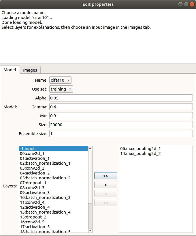
At the bottom left of the window, you see a list of layers of the model that are available for explanations. Pooling layers 6 and 14, shown on the right, have been pre-selected. You can move layers into or out of this list by selecting them and using the < and > buttons.

Click the Images tab. This will show you a collection of the first 50 training images in the dataset that the model classifies as airplanes (classification 0):

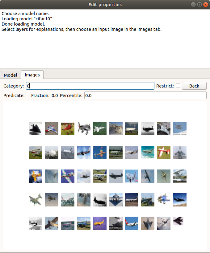
Notice that the sixth image in the first row is actually an image of a cat that the network has mis-classified. Let’s try to understand what features of this image caused it to be mis-classified. Click on the image to select it. You will see a larger version of the image. Click on this larger version to compute an explanation.

Computing the explanation will take about 20 seconds on an ordinary CPU, because nnitp first has to evaluate the model over a large collection of images. When the computation is finished, you will see a message like this:

Interpolant: layer 14: (v(0,4,25)<=-0.69624305 & v(5,0,44)>=1.063251 & v(6,3,62)>=0.53659225 & v(4,6,34)>=3.1080968 & v(4,7,8)>=-0.6518301)
On training set: F = 1, N = 67, P = 1954, precision=0.9850746268656716, recall=0.033776867963152504
On test set: F = 5, N = 39, P = 980, precision=0.8717948717948718, recall=0.03469387755102041

Nnitp has computed an interpolant at layer 14. This is a fact about the activation of the layer for this image that predicts a classification of airplane with fairly high precision. That is, given interpolant condition, the probability of a test set image being classified as an airplane is 0.985, while the probability over test set images is 0.872. Because the interpolant was learned over the training set, it’s the test set precision that counts. The recall of the interpolant is about 3.5%. This means that about 3.5% of the images classified as airplanes satisfied this condition.

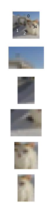
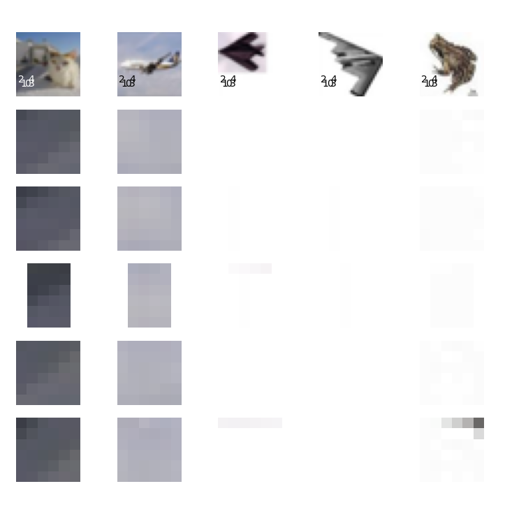
The interpolant is a logical and of five constraints on unit activations. For example, the constraint v(0,4,25)<=-0.696 tells us that the activation of channel 25 at image coordinate position (0,4) is less than or equal to -0.696. This fact is not very helpful to begin with, since we don’t know what features of the image these units represent. To give a better idea, nnitp displays a grid of images. In the column on the left, we see our cat image, and, below it, the five regions of the image that affected the five neural net units in the interpolant. Superimposed on the top image are digits 0–4 placed at the location of the corresponding unit:

The remaining columns of the image grid are comparison images. These are images that also happen to satisfy the interpolant condition. In each row, we see the image region that affects the corresponding constraint:

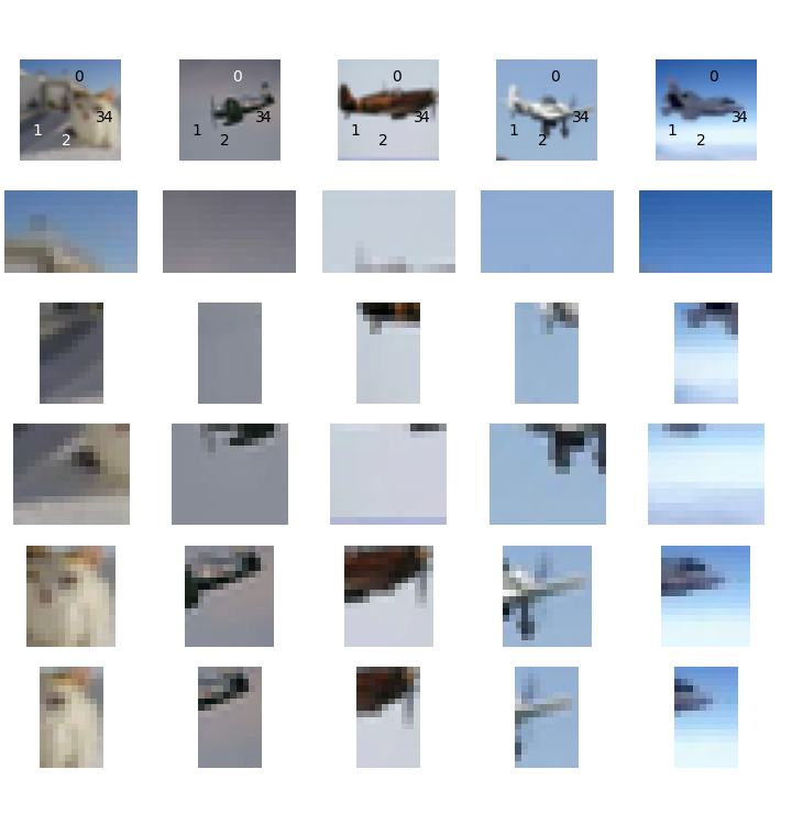
We can already begin to see why the network thinks the cat is an airplane. Regions 0–2 correspond to mostly empty space in all of the images. On the other hand, regions 3–4 contain a diagonal feature in the true airplane images.

To understand why the cat also has these features, let’s look for explanations of some of the individual constraints. As an example, the image in the left column, third row, satisfies constraint 1. It is a gray region with some diagonal streaks. Click on that image to get an explanation of why it satisfies condition 1. This time, we got very good precision of the interpolant: it is a fact about layer 6 that predicts the feature at layer 14 with 97.6% probability over the test set.

Here is part of the resulting image grid:

The regions used in the constraints five constraints have fewer pixels because layer 6 is closer to the input image. By comparing to the columns at right, we see that this feature is just recognizing blank space. Notice that one of the comparison images satisfying this interpolant is actually a frog surrounded by blank space.

Now click the back button, to go back to our origin interpolant at layer 14. Click on the image in the left column, fifth row, that shows the cat’s face. Again, we get an interpolant with pretty high precision: 98%. Here is part of the grid:

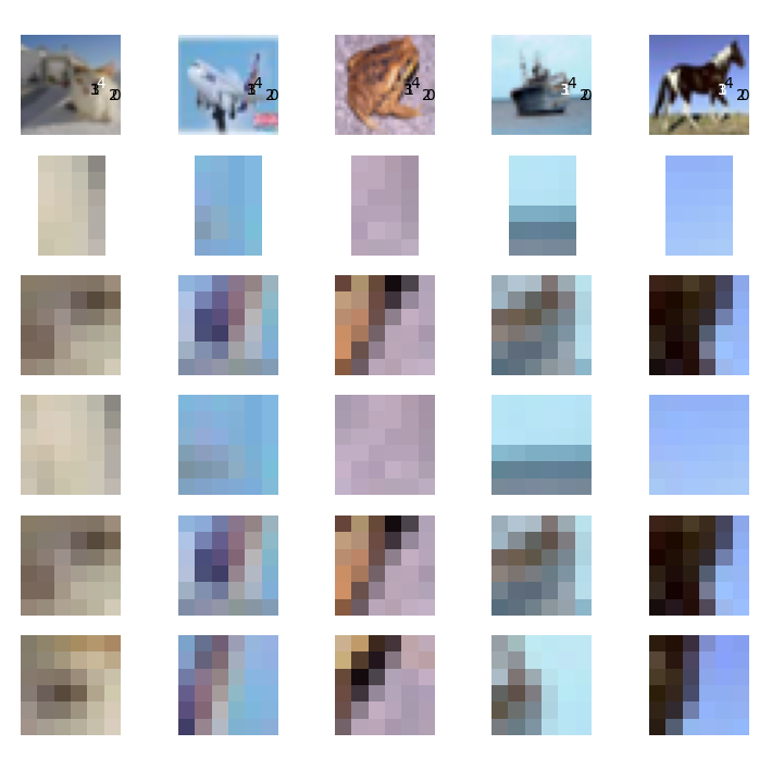
What’s in common to these images, including a frog, a ship and a horse, is that they contain diagonal feature, with some blank space around it. In the case of the cat, the diagonal feature runs between the nose and the left eye of the cat. In effect, the net has confused the face of the cat with the tail or wing of a plane.

It’s clear that the network is not recognizing shapes in the sense that we normally think of them, as connected objects. The network has learned that a single diagonal feature with a lot of blank space around it is sufficient to distinguish an airplane, and this has resulted in incorrectly classifying an image of a cat that happens to have these features as an airplane. Perhaps this means that we should add images of airplanes over more varied backgrounds to the training set.

It’s also interesting to note that the individual units within the network are nearly uninterpretable as features. To get a sense of this, left-click on the image of that cat’s face in the left column, row three, and select the menu item Examples. This will show some images that satisfy the interpolant’s constraint on just one unit. Here’s some of what we see:

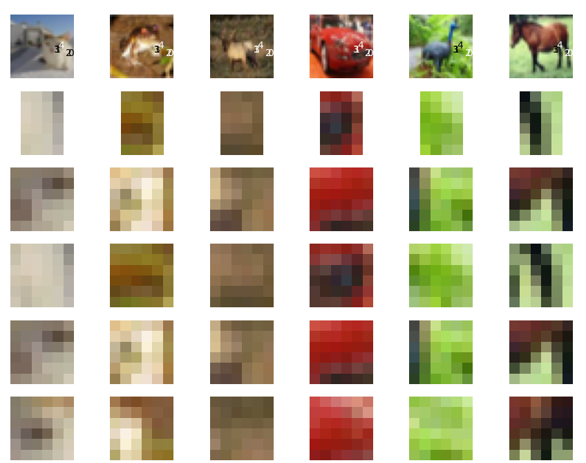
Some image regions in the third row do indeed contain a diagonal edge, but its very hard to generalize about these image fragments. This seems to be generally true about neural nets: an individual hidden unit is a very noisy predictor. We need to collect an ensemble of units to recognize a meaningful feature.